Introduction to the User Interface
Warning
The user interface referenced below has been deprecated.
Starting the Jupyter Hub
During the hackathon we will be using the user interface (UI) located here.
You will need to log in with your Github username and password
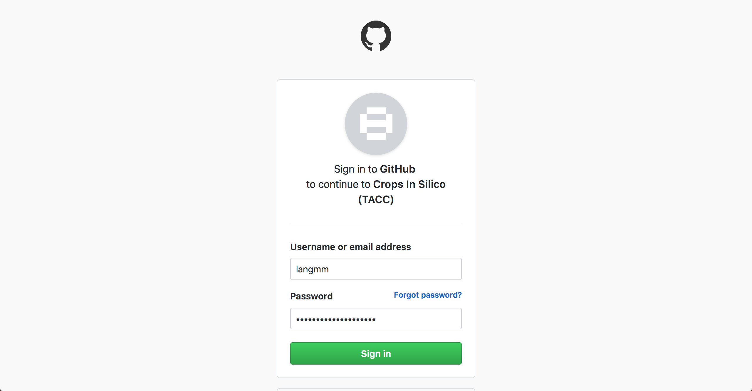
and then start a server.
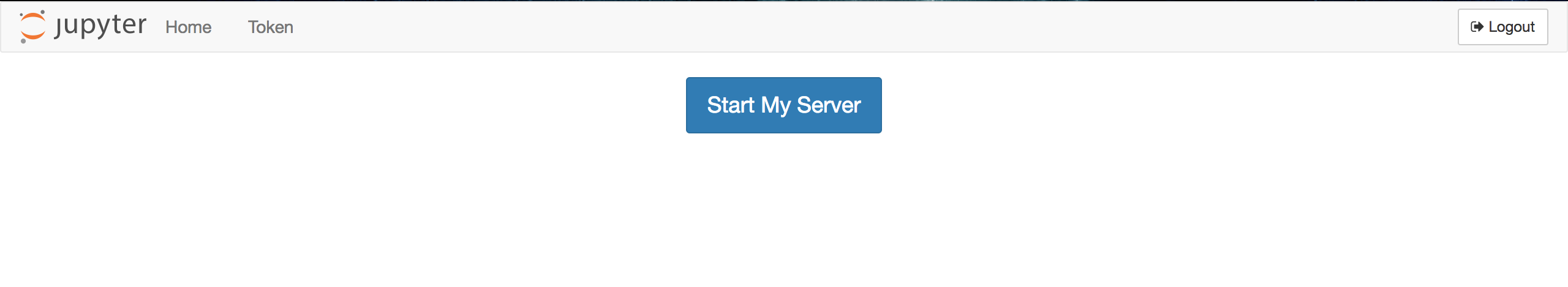
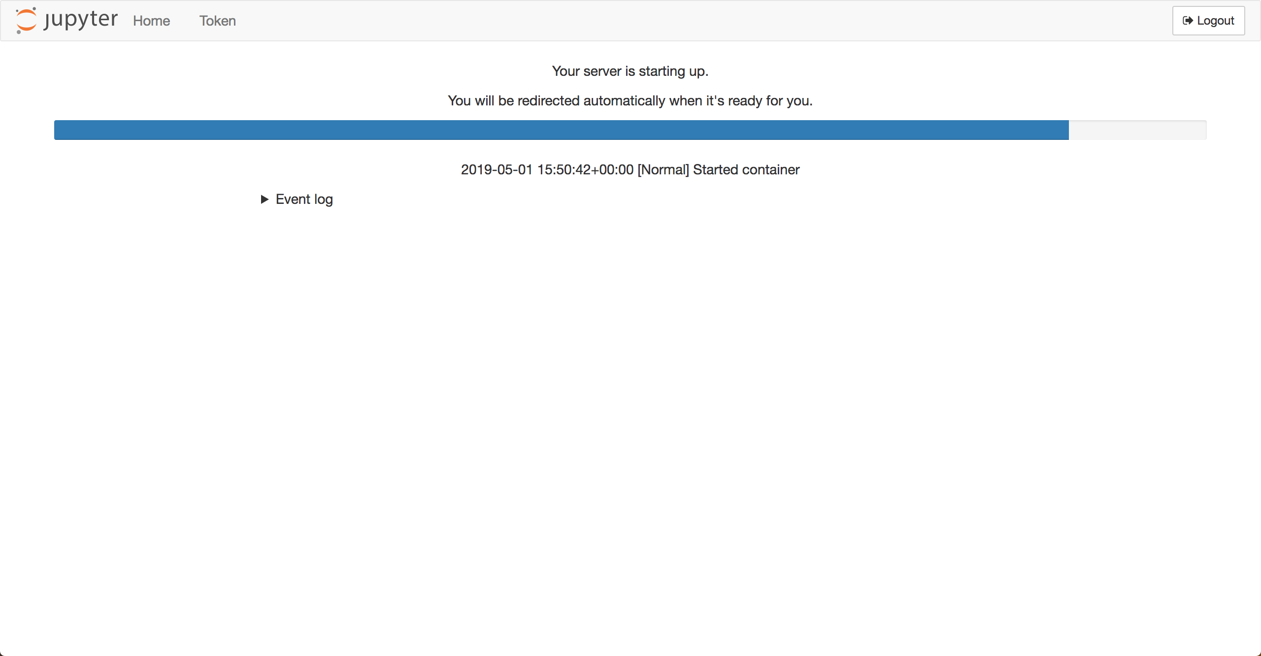
This may take a moment.
Orientation
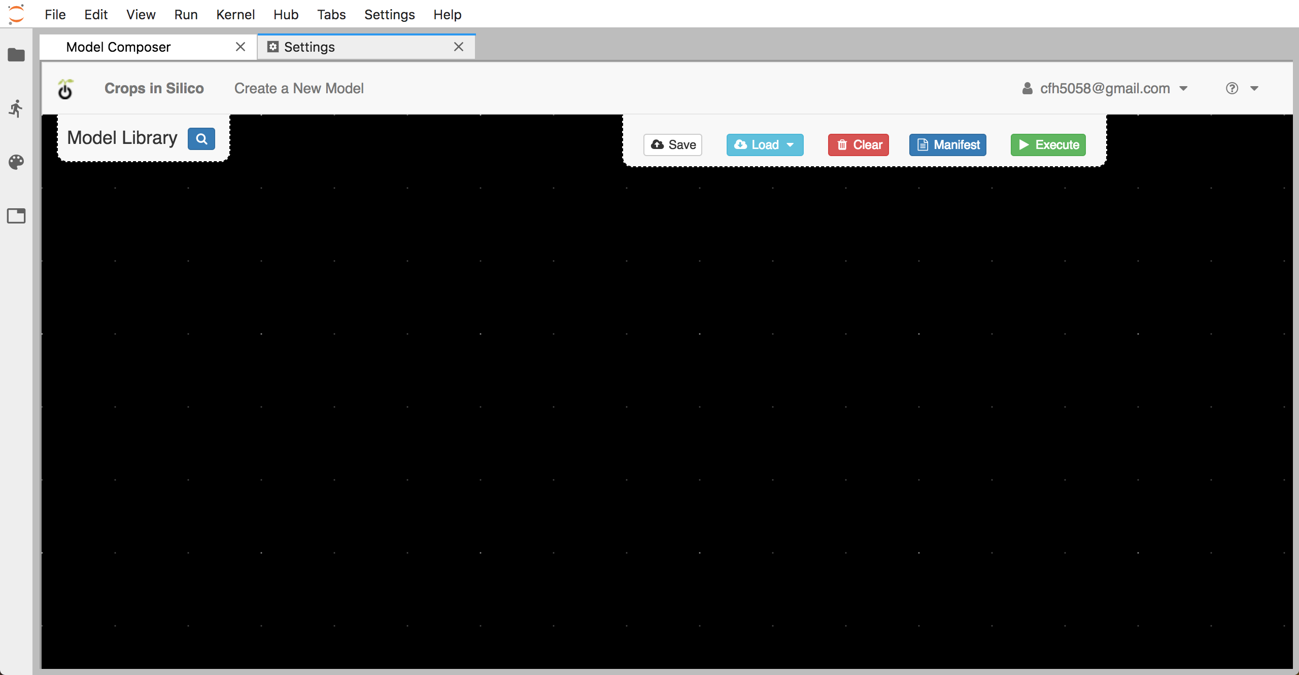
Once the server is started, you will see a Jupyter hub interface that includes
a Model Composer tab. Within the Model Composer tab you have a canvas (the black
area), a model palette titled Model Library in the upper left corner of the canvas
that is populated with examples models from a dedicated model repository, and several
actions buttons in the upper right corner of the canvas. The Save button will save
graphs to your workspace, the Load button provides a drop-down menu of several
pre-defined graphs containing the models listed in the model palette that can be loaded
into the canvas, the Clear button will clear any models/connections from the canvas,
the Manifest button will display the YAML file required to run the currently loaded
graph locally, and the Execute button will run the currently loaded graph (assuming
the models are loaded into the workspace).
Loading & Running an Existing Integration
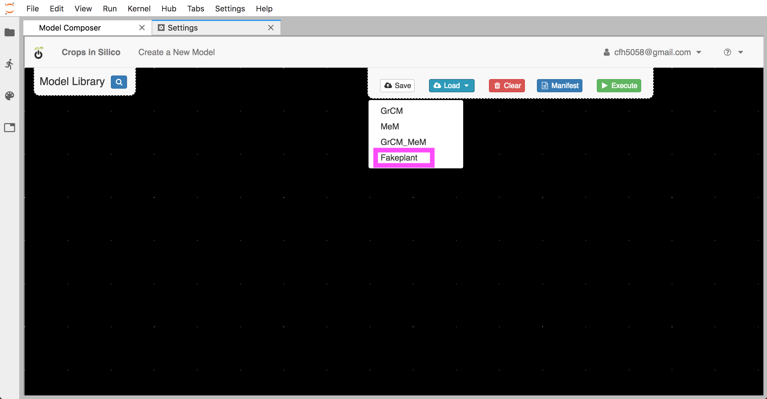
First we will load and execute an existing integration graph that is pre-loaded into
the Jupyter hub. From the Load drop down menu, select the Fakeplant option to
load an example integration network that uses the models from the hackathon2019
repository that we cloned in preparation.
Once loaded you will see several icons connected with white lines that represents 4 models connected to 6 input files.
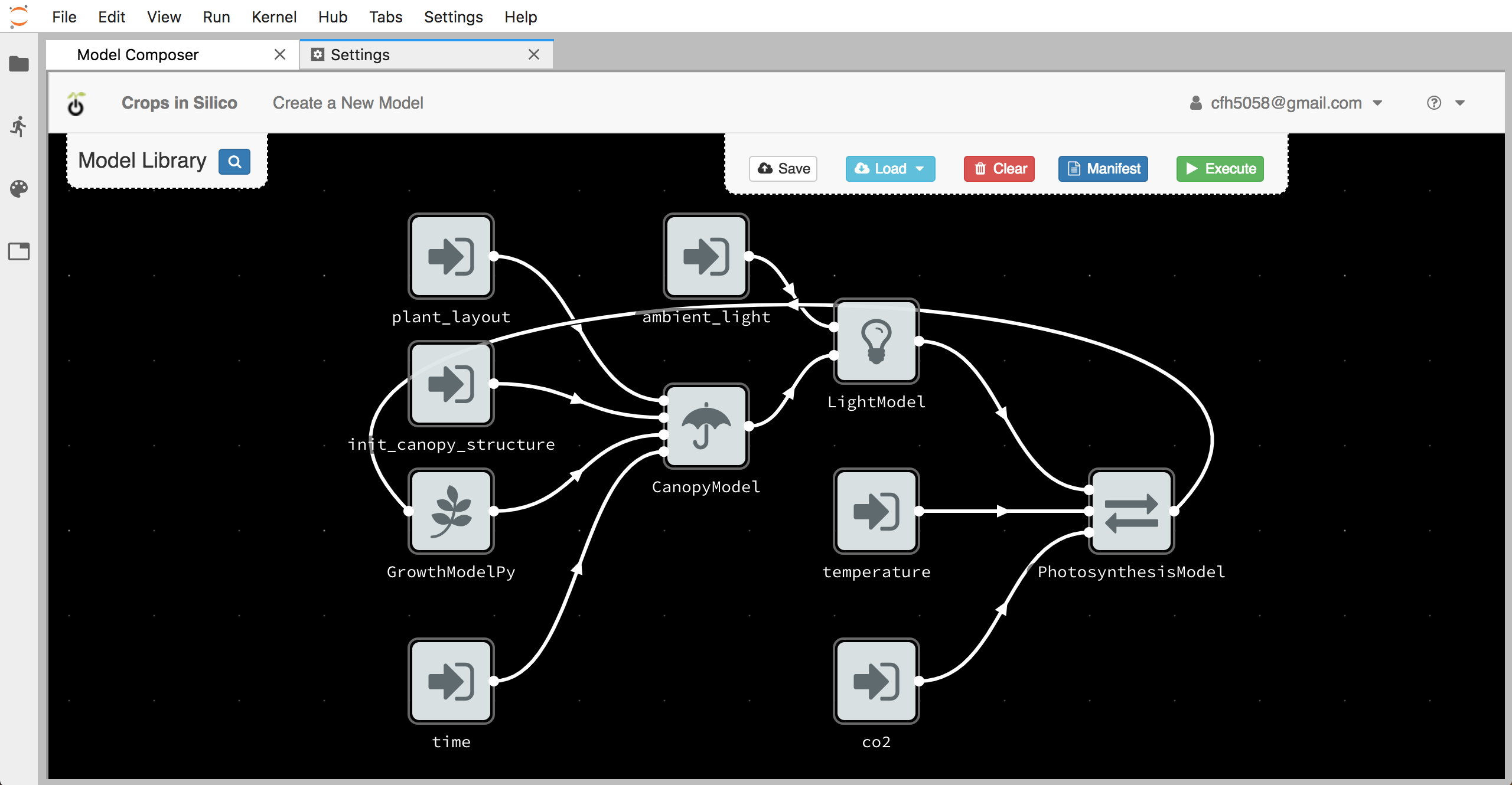
Each icon represents one of the models in the hackathon2019
repository that you cloned to your local machine or an input/output file.
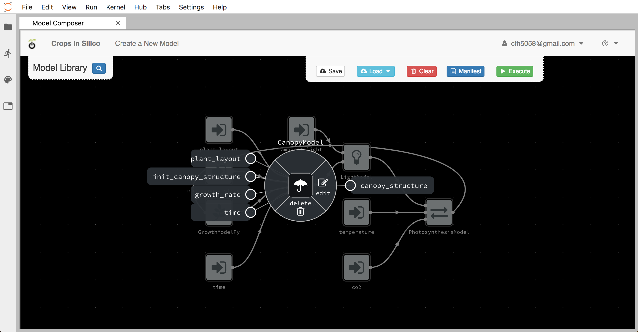
By right clicking on each model, you can get information about the model’s
inputs and outputs.
The canopy model takes as input an initial canopy structure, a growth rate, a plant layout describing how the plant grows in x, y, and z, and a time step. From this information it grows the canopy structure and outputs the updated structure. The canopy model is written in C++.
The light model takes as input an ambient light level and the 3D structure of the canopy. It then calculates the light incident on each facet of the canopy structure which it outputs.
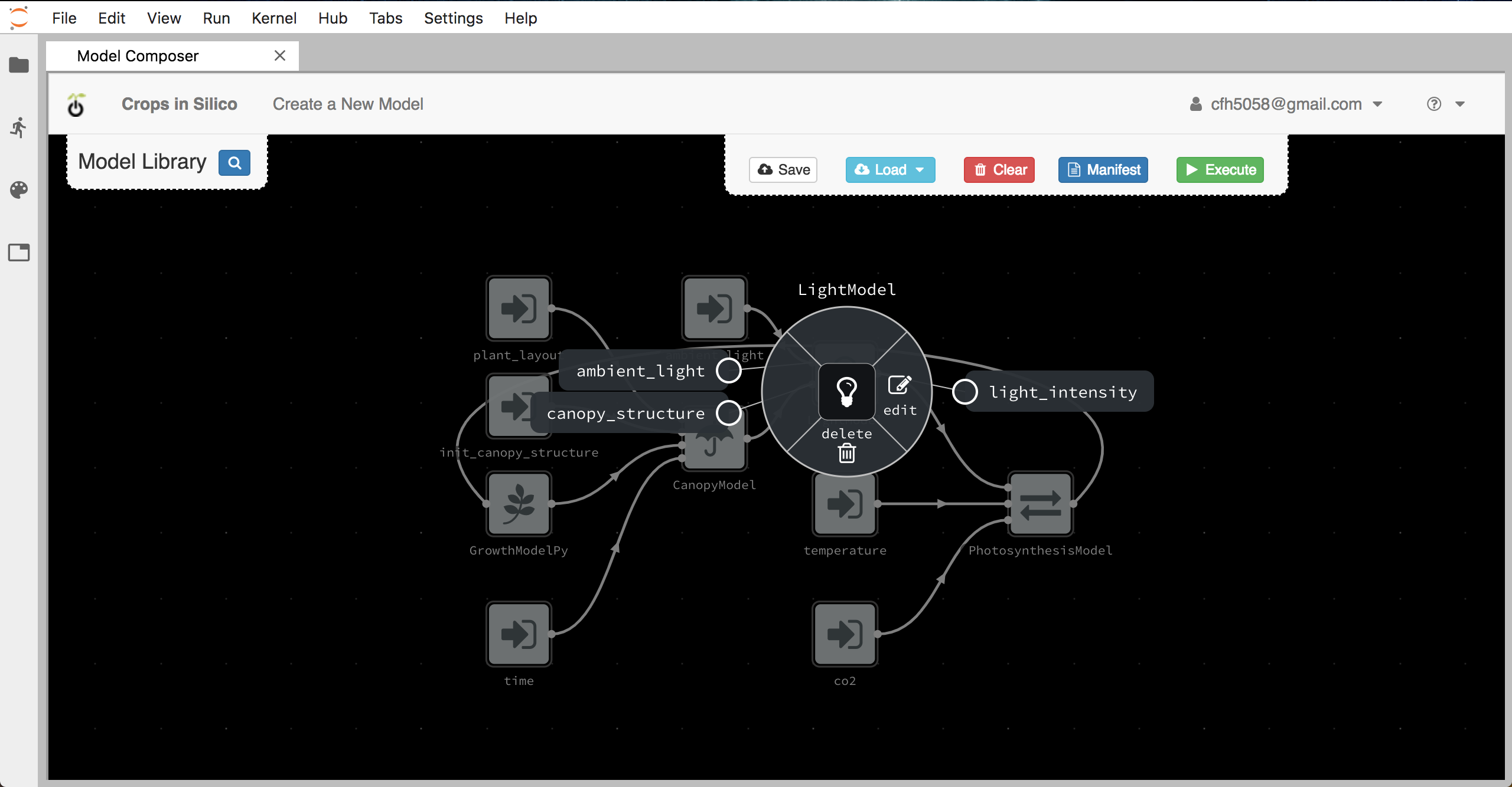
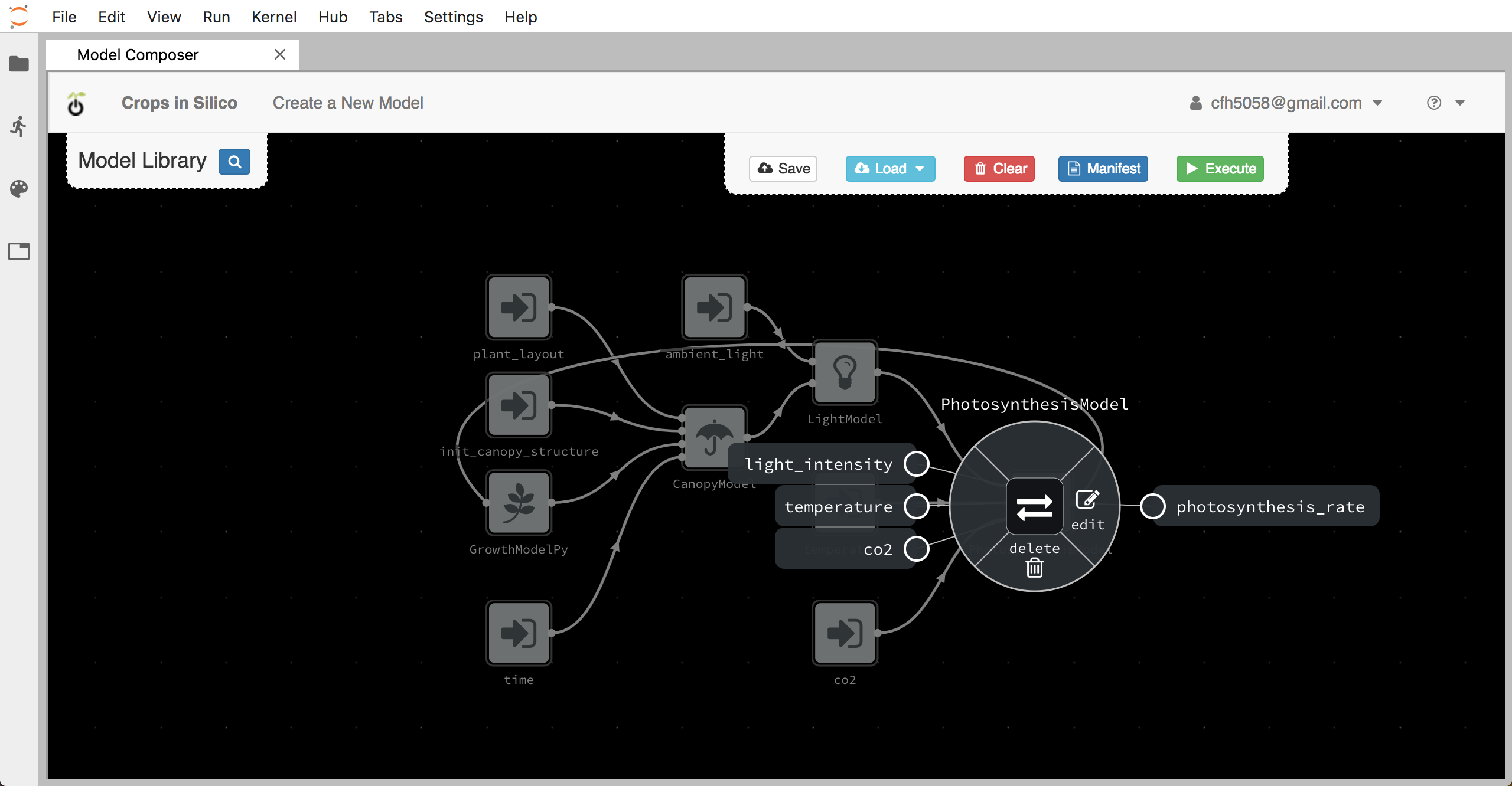
The photosynthesis model takes as input a light intensity, temperature, and CO2. From this information, it calculates and output the photosynthesis rate.
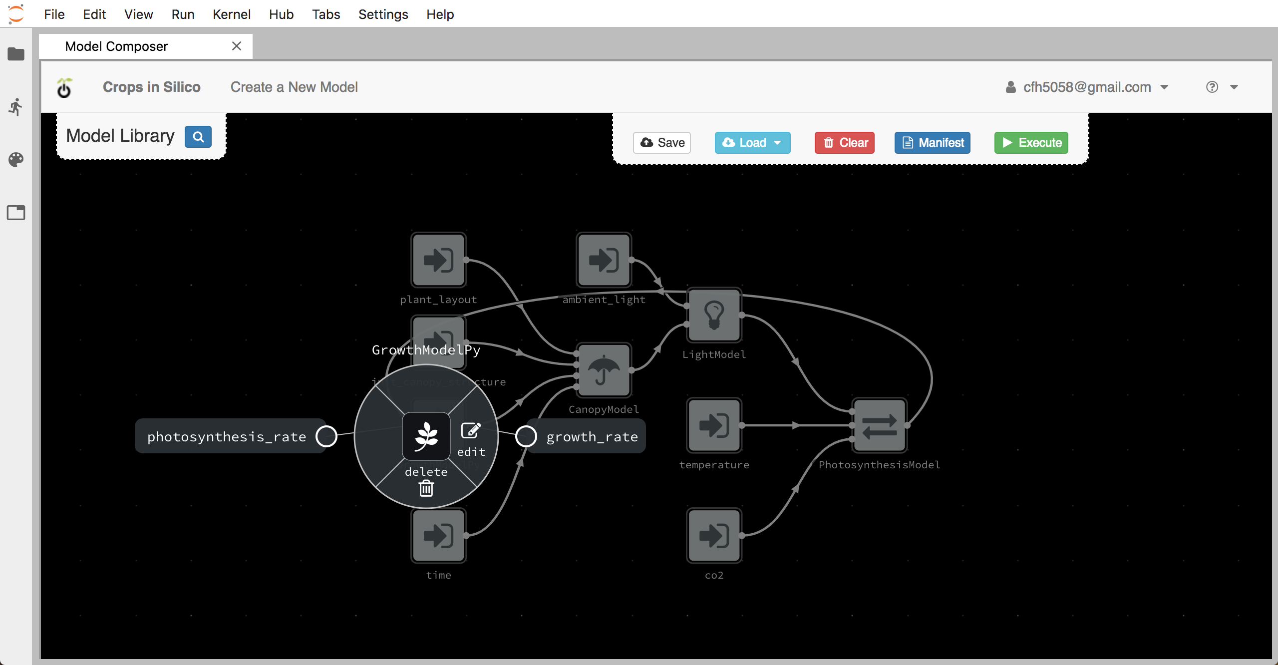
The growth model in this network is an alternative to the growth model we were working with in the previous section. It takes photosynthesis rate as an input and outputs the growth rate. We will be replacing this growth model with the one you created.
You can trace the data as it flows from files and from one model to the next.
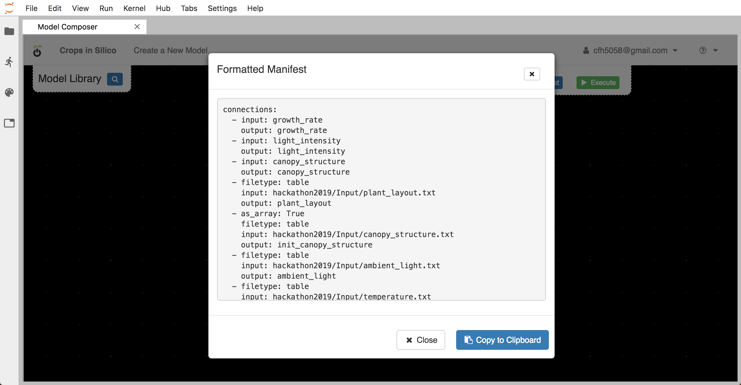
You can view the
YAML generated from the integration graph by clicking the Manifest button.
You can run the integration by clicking the Execute button. Once the models begin
running, a window display the output log will pop up.
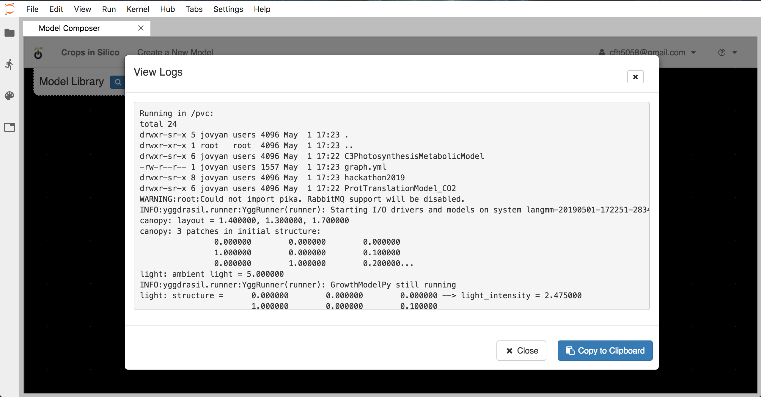
The output log will include log messages from yggdrasil about the model execution intermingled with output from the models themselves. Because the model run in parallel and communication output at different rates, the model output may or may not be sequential.
In the next we will integrate a new growth model and add it to this integration network as a replacement for the existing growth model.